At each voxel/vertex/face/edge we have a linear model expressed as:
\[\mathbf{Y} = \mathbf{M} \boldsymbol{\psi} + \boldsymbol{\epsilon}\]
or equivalently as:
\[\mathbf{Y} = \mathbf{X}\boldsymbol{\beta} + \mathbf{Z}\boldsymbol{\gamma} + \boldsymbol{\epsilon}\]
where \(\mathbf{X}\) contains the regressors of interest and \(\mathbf{Z}\) the nuisance regressors, with the remaining as usual. For a linear null hypothesis \(\mathcal{H}_0 : \mathbf{C}'\boldsymbol{\psi}=\boldsymbol{\beta}=\mathbf{0}\), the \(t\) statistic can be computed as:
\[t = \boldsymbol{\hat{\psi}}'\mathbf{C} \left(\mathbf{C}'(\mathbf{M}'\mathbf{M})^{-1}\mathbf{C} \right)^{-\frac{1}{2}} \left/ \sqrt{\dfrac{\boldsymbol{\hat{\epsilon}}'\boldsymbol{\hat{\epsilon}}}{N-\mathsf{rank}\left(\mathbf{M}\right)}} \right.\]
whereas the \(F\) statistic can be computed as:
\[\begin{array}{ccl} F &=& \left.\dfrac{\boldsymbol{\hat{\psi}}'\mathbf{C} \left(\mathbf{C}'(\mathbf{M}'\mathbf{M})^{-1}\mathbf{C} \right)^{-1} \mathbf{C}'\boldsymbol{\hat{\psi}}}{\mathsf{rank}\left(\mathbf{C}\right)} \right/ \dfrac{\boldsymbol{\hat{\epsilon}}'\boldsymbol{\hat{\epsilon}}}{N-\mathsf{rank}\left(\mathbf{M}\right)}\\[15pt] {} & = & \left.\dfrac{\boldsymbol{\hat{\beta}}' \left(\mathbf{X}'\mathbf{X}\right)\boldsymbol{\hat{\beta}}}{\mathsf{rank}\left(\mathbf{C}\right)} \right/ \dfrac{\boldsymbol{\hat{\epsilon}}'\boldsymbol{\hat{\epsilon}}}{N-\mathsf{rank}\left(\mathbf{X}\right)-\mathsf{rank}\left(\mathbf{Z}\right)} \end{array}\]
We assess the significance of the statistic by repeating the same fit after shuffling \(\mathbf{Y}\), \(\mathbf{X}\) or \(\mathbf{M}\), or variations of these, recalculating the statistic and building its distribution, from which the p-values are obtained (well, not really...).
Shuffling is only allowed if it doesn't affect the distribution of the error terms, i.e., if the errors are exchangeable.
A blast from the past... Tom et al 2008 HBM poster:
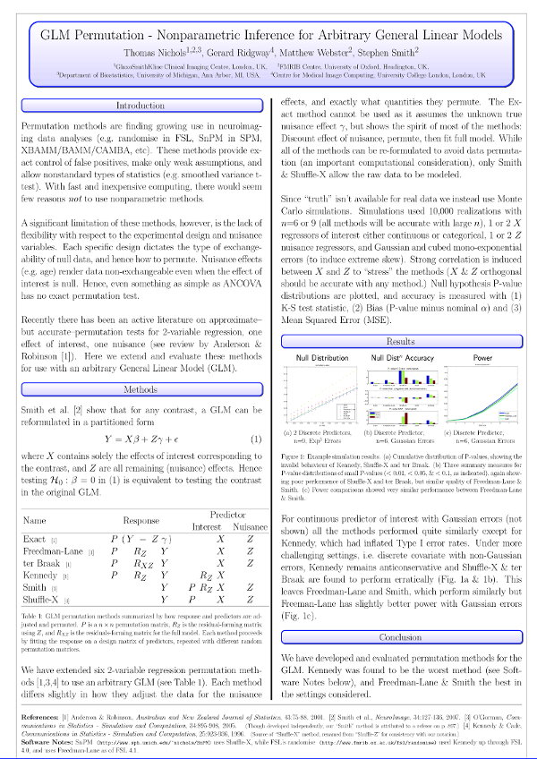
We extended these evaluations to include other methods, and presented all in a common notation to allow direct visual comparison:
| Method | Model |
|---|---|
| Draper-Stoneman (1966) | \(\mathbf{Y}=\mathbf{P}\mathbf{X}\boldsymbol{\beta} + \mathbf{Z}\boldsymbol{\gamma} + \boldsymbol{\epsilon}\) |
| Still-White (1981) | \(\mathbf{P}\mathbf{R}_{\mathbf{Z}}\mathbf{Y}=\mathbf{X}\boldsymbol{\beta} + \boldsymbol{\epsilon}\) |
| Freedman-Lane (1983) | \(\left(\mathbf{P}\mathbf{R}_{\mathbf{Z}}+\mathbf{H}_{\mathbf{Z}}\right)\mathbf{Y}=\mathbf{X}\boldsymbol{\beta} + \mathbf{Z}\boldsymbol{\gamma}+\boldsymbol{\epsilon}\) |
| Manly (1986) | \(\mathbf{P}\mathbf{Y}=\mathbf{X}\boldsymbol{\beta} + \mathbf{Z}\boldsymbol{\gamma} + \boldsymbol{\epsilon}\) |
| ter Braak (1988) | \(\left(\mathbf{P}\mathbf{R}_{\mathbf{M}}+\mathbf{H}_{\mathbf{M}}\right)\mathbf{Y}=\mathbf{X}\boldsymbol{\beta} + \mathbf{Z}\boldsymbol{\gamma}+\boldsymbol{\epsilon}\) |
| Kennedy (1996) | \(\mathbf{P}\mathbf{R}_{\mathbf{Z}}\mathbf{Y}=\mathbf{R}_{\mathbf{Z}}\mathbf{X}\boldsymbol{\beta} + \boldsymbol{\epsilon}\) |
| Huh-Jhun (2001) | \(\mathbf{P}\mathbf{Q}'\mathbf{R}_{\mathbf{Z}}\mathbf{Y}=\mathbf{Q}'\mathbf{R}_{\mathbf{Z}}\mathbf{X}\boldsymbol{\beta} + \boldsymbol{\epsilon}\) |
| Smith (2008) | \(\mathbf{Y}=\mathbf{P}\mathbf{R}_{\mathbf{Z}}\mathbf{X}\boldsymbol{\beta} + \mathbf{Z}\boldsymbol{\gamma} + \boldsymbol{\epsilon}\) |
| Parametric (1918) | \(\mathbf{Y}=\mathbf{X}\boldsymbol{\beta} + \mathbf{Z}\boldsymbol{\gamma} + \boldsymbol{\epsilon},\;\; \boldsymbol{\epsilon}\sim\mathcal{N}(0,\sigma^2\mathbf{I})\) |
After thorough evaluation, the conclusion was that the Freedman-Lane and Smith are the best methods in a diverse set of scenarios, with the best control over the error rate and generally higher power.
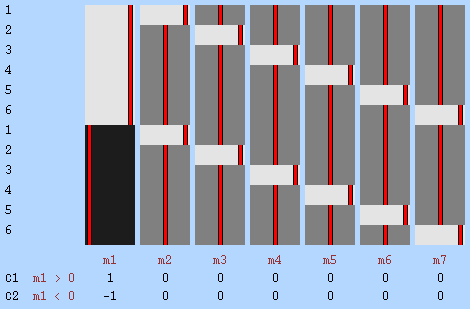
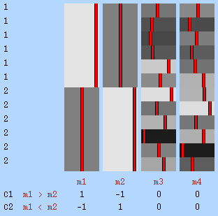
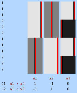
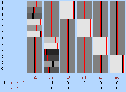
The shuffling strategy in these methods can be represented by permutation matrix \(\mathbf{P}\). This matrix can incorporate permutations, sign-flippings, or both:
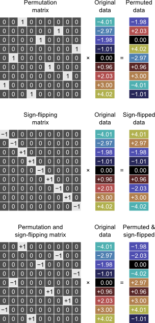
Shuffling can be seen as replacing the observed data (or design) for other data that possesses the exact same properties. If we knew precisely what these properties were, we could do Monte Carlo (or even parametric), but since we don't know, we replace instead for the best estimate that we have, which is the data itself.
Unrestricted permutations can be used when:
- The errors cannot assumed to be distributed normally;
- The errors may not be independent, but are still exchangeable.
Unrestricted sign-flips can be used when:
- The errors may not be distributed normally, but at least are symmetric;
- The errors are independent.
Unrestricted permutations and sign-flips can be used:
- When the conditions above overlap, i.e., when the distributions are symmetric and independent.
- An alternative to permutation and/or sign-flipping alone when there are too few permutations.
Advantages of permutation tests
- At each individual test, weaker and tenable assumptions about the data.
- For multiple tests, easy correction for familywise error rate (FWER), without the need to know how the tests are related to each other.
- The same permutation framework can be used for virtually all experimental modalities (imaging or not).
- Does not rely on random sampling of an imaginary, infinite population, but on more realistic random allocation of experimental units. Results can still be generalised to population if the sampling is unbiased.
Disadvantages of permutation tests
- Computationally intensive.
- Discrete p-values only (sometimes this is a problem).
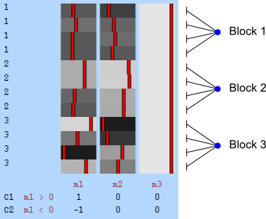
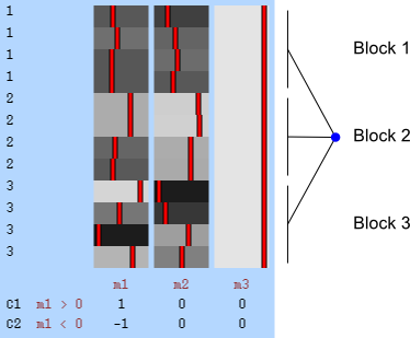
In some studies, the observations themselves may not be exchangeable, but sets (blocks) of them might be. This is the case, for instance, of designs that involve repeated measurements. Two kinds of shuffling are possible:
- Within block: the observations are shuffled inside the block only, never across blocks.
- Whole block: the blocks of observations are shuffled as a whole, keeping the relative order of the observations inside unaltered.
Within-block permutation is available in randomise with the specification of the exchangeability blocks file with the option -e. Whole-block is also available if, in addition to the option -e, the option --permuteBlocks is supplied.
The presence of exchangeability blocks imply that observations cannot be pooled together to produce a non-linear parameter estimate such as the variance. In other words: the mere presence of exchangeability blocks, either for shuffling within or as a whole, implies that the variances may not be the same across all observations, and a single estimate of this variance is likely to be inaccurate if the variances truly differ, or if the groups don't have the same size. This also means that the \(F\) or \(t\) statistics may not behave as expected.
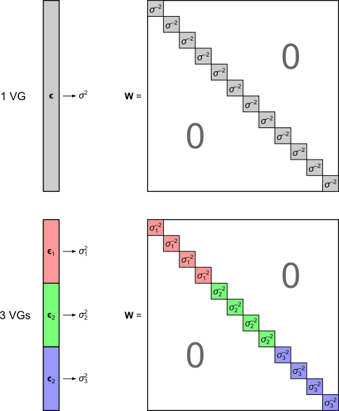
The solution is to use the block definitions and the permutation strategy to define groups of observations that are known or assumed to have identical variances, and pool only the observations within group for variance estimation, i.e., to define variance groups (VGs).
The \(F\)-statistic, however, doesn't allow such multiple groups of variances. The solution is to use another statistic. The proposal here is to define:
\[G = \dfrac{\boldsymbol{\hat{\psi}}'\mathbf{C} \left(\mathbf{C}'(\mathbf{M}'\mathbf{W}\mathbf{M})^{-1}\mathbf{C} \right)^{-1} \mathbf{C}'\boldsymbol{\hat{\psi}}}{\Lambda \cdot s}\]
where \(\mathbf{W}\) is a diagonal matrix that has elements:
\[W_{nn}=\dfrac{\sum_{n' \in g_{n}}R_{n'n'}}{\boldsymbol{\hat{\epsilon}}_{g_{n}}'\boldsymbol{\hat{\epsilon}}_{g_{n}}}\]
\[\Lambda = 1+\frac{2(s-1)}{s(s+2)}\sum_{g} \frac{1}{\sum_{n \in g}R_{nn}} \left(1-\frac{\sum_{n \in g}W_{nn}}{\mathsf{trace}\left(\mathbf{W}\right)}\right)^2\]
and where \(s=\mathsf{rank}\left(\mathbf{C}\right)\). The matrix \(\mathbf{W}\) can be seen as a weighting matrix, the square root of which normalises the model such that the errors have then unit variance and can be ignored.
When \(\mathsf{rank}\left(\mathbf{C}\right)=1\), the \(t\)-equivalent to the \(G\)-statistic is \(v = \boldsymbol{\hat{\psi}}'\mathbf{C} \left(\mathbf{C}'(\mathbf{M}'\mathbf{W}\mathbf{M})^{-1}\mathbf{C} \right)^{-\frac{1}{2}}\), which is the same \(v\)-statistic for the Behrens-Fisher problem.
In the absence of variance groups (i.e., all observations belong to the same VG), \(G\) and \(v\) are equivalent to \(F\) and \(t\) respectively.
Although not typically necessary, approximate parametric p-values for the \(G\)-statistic can be computed from an \(F\)-distribution with \(\nu_1=s\) and \(\nu_2=2(s-1)/3/(\Lambda-1)\).
The \(G\)-statistic has a fixed distribution even under unequal variances — this is what it was made for! And it's more powerful (see Table 6 in the paper, page 31).
Example 3: Paired t-test — Consider a study to investigate the effect of the use of a certain analgesic in the magnitude of the BOLD response associated with painful stimulation. In this example, the response after the treatment is compared with the response before the treatment, i.e., each subject is their own control. The experimental design is the "paired \(t\)-test". One EB is defined per subject, as the observations are not exchangeable freely across subjects, and must remain together in all permutations. In this example, in the absence of evidence on the contrary, the variance was assumed to be homogeneous across all observations, such only one VG, encompassing all, was defined. If instead of just two, three or more observations per subject were being compared, the same strategy, with the necessary modifications to the design matrix, could be applied only under the assumption of compound symmetry, something clearly invalid for most studies, albeit not for all. Some designs with repeated measurements can, however, bypass this need altogether, as shown in Example 6.
Example 4: Unequal group variances — Consider a study using FMRI to compare whether the BOLD response associated with a certain cognitive task would differ among subjects with autistic spectrum disorder (ASD) and control subjects, while taking into account differences in age and sex. In this hypothetical example, the cognitive task is known to produce more erratic signal changes in the patient group than in controls. Therefore, variances cannot be assumed to be homogeneous with respect to the group assignment of subjects. This is an example of the classical Behrens-Fisher problem. To accommodate heteroscedasticity, two permutation blocks are defined according to the group of subjects. Under the assumption of independent and symmetric errors, the problem is solved by means of random sign-flipping, using the well known Welch's \(v\) statistic, a particular case of the statistic \(G\).
Example 5: Variance as a confound — Consider a study using FMRI to compare whether a given medication would modify the BOLD response associated with a certain attention task. The subjects are allocated in two groups, one receiving the drug, the other not. In this hypothetical example, the task is known to produce very robust and, on average, similar responses for male and female subjects, although it is also known that males tend to display more erratic signal changes, either very strong or very weak, regardless of the drug. Therefore, variances cannot be assumed to be homogeneous with respect to the sex of the subjects. To accommodate heteroscedasticity, two permutation blocks are defined according to sex, and each permutation matrix is constructed such that permutations only happen within each of these blocks.
Example 6: Longitudinal study — Consider a study to evaluate whether fractional anisoptropy (FA) would mature differently between boys and girls during middle childhood. Each child recruited to the study is examined three times, at the ages of 9, 10 and 11 years, and none of them are related in any known way. Permutation of observations within child cannot be considered, as the null hypothesis is not that FA itself would be zero, nor that there would be no changes in the value of FA along the three yearly observations, but that there would be no difference in potential changes between the two groups; the permutations must, therefore, always keep in the same order the three observations. Moreover, with three observations, it might be untenable to suppose that the joint distribution between the first and second observations would be the same as for between first and third, even though it might be the same as for the second and third; if these three pairwise joint distributions cannot be assumed to be the same, this precludes within-block exchangeability. Instead, blocks are defined as one per subject, each encompassing all the three observations, and permutation of each block as a whole is performed. It is still necessary, however, that the covariance structure within block (subject) is the same for all blocks, preserving exchangeability. If the variances cannot be assumed to be identical along time, one variance group can be defined per time point, otherwise all are assigned to the same VG (as in Example 3). If there are nuisance variables to be considered (some measurements of nutritional status, for instance), these can be included in the model and the procedure is performed using the same Freedman-Lane or Smith strategies.

Definition
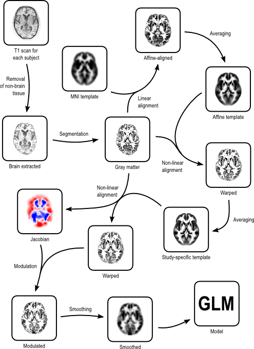
VBM (Voxel-Based Morphometry) is a method used to study the amount of gray matter contained in each voxel and compare across subjects.
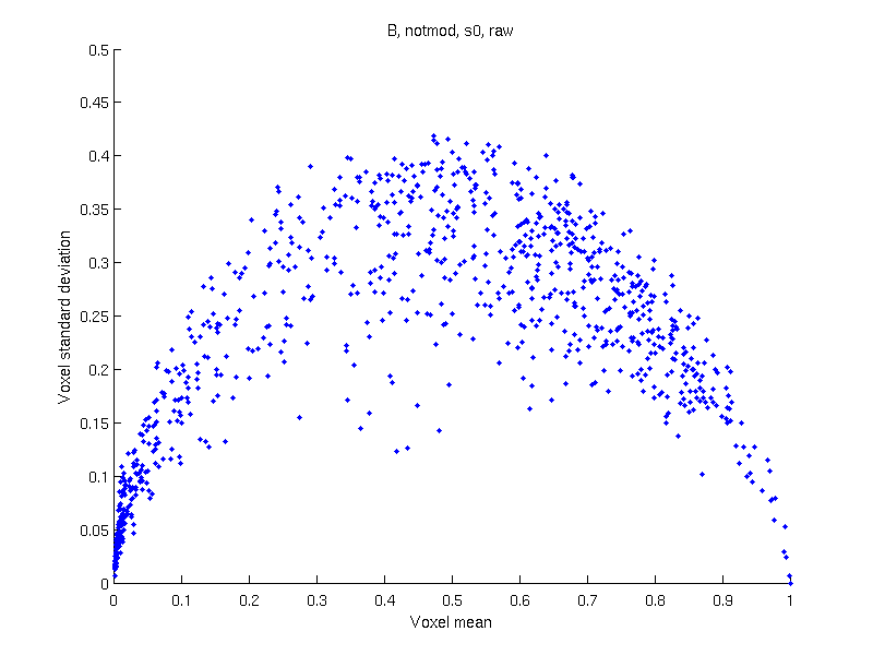
Problems
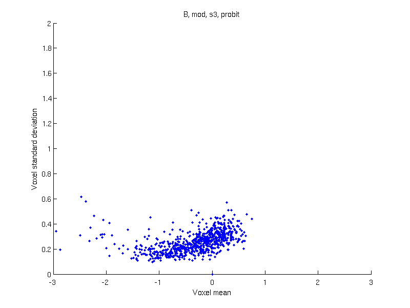
Several potential issues may affect VBM, and on what concerns this discussion, the variance is not independent of the mean. The consequence is that, whenever there are difference in means (the exact objective of the method) there will also be difference in variances, invalidating most parametric, but also permutation tests, given the pivotality issues just discussed.
| Without smoothing | With smoothing | |
|---|---|---|
| Without modulation | |
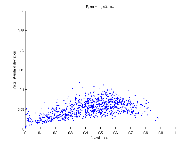 |
| With modulation |  |
 |
Suggested solutions
These issues can be solved by:
Use the \(G\)-statistic — Defining one exchangeability block per experimental group and shuffling within block only. Each block corresponds to its own variance group. Use the \(G\)-statistic assessed via permutations.
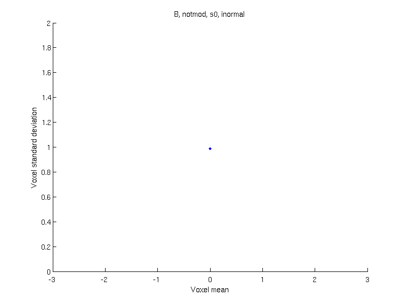
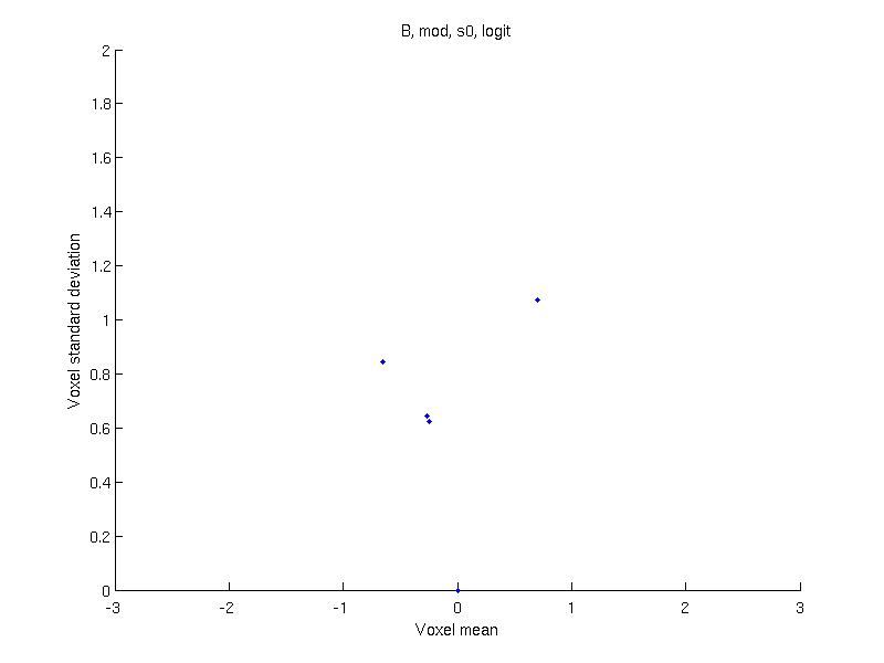
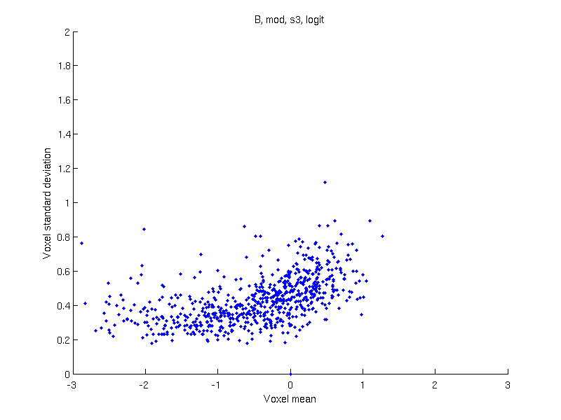
Apply a data transformation — If after the above, only sign-flipping can be used, apply a data transformation, such as logit (as in the original Ashburner & Friston 2000 paper) or probit.
Alternatively, some transformations (e.g., rank-based inverse-normal) may render the definition of exchangeability groups no longer necessary, and VBM can proceed as usual. The same can be used to other methods that may suffer from similar issues, e.g., FA data, etc.
| Logit | Probit | Inverse normal |
|---|---|---|
| \(\tilde{Y}=\log\left(\dfrac{Y}{1-Y}\right)\) | \(\tilde{Y}=\Phi^{-1}\left\{1-Y\right\}\) | \(\tilde{Y}=\Phi^{-1}\left\{\dfrac{r_i}{n+1}\right\}\) |
Results
| Logit | Probit | Inverse normal | ||||
|---|---|---|---|---|---|---|
| Without smoothing | With smoothing |
Without smoothing | With smoothing |
Without smoothing | With smoothing |
|
| Without modulation |
 |
 |
 |
 |
 |
 |
| With modulation |
 |
 |
 |
 |
 |
 |
Hamming R. Error detecting and error correcting codes. Bell Syst Tech J. 1950;29(2):147-160.
Horn S, Horn R, Duncan D. Estimating heteroscedastic variances in linear models. J Am Stat Assoc. 1975;70(350):380-385.
Pesarin F. A new solution for the generalized Behrens-Fisher problem. Statistica. 1995;50(2):131-146.
Welch B. On the comparison of several mean values: an alternative approach. Biometrika. 1951;38(3):330-336.
Winkler AM, Ridgway GR, Webster MA, Smith SM, Nichols TE. Permutation inference for the general linear model. Neuroimage. 2014 [Epub ahead of print]