Surface Analysis
Surface analysis comprises techniques that allow you to inspect smooth surfaces and to detect any imperfections or discontinuities that may exist. In form•Z, surface analysis is an attribute that stays with an object and can be displayed during all modeling and editing operations, while the object is displayed using the Shaded Work rendering mode.
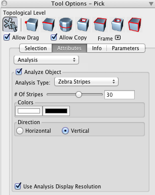
The Analysis tab in the tool options palette.
To apply a surface analysis to an object, first display it in Shaded Work mode. Then use the Pick tool to select it and in the Pick Tool Options palette open the Attributes tab. From the popup menu at the top of the tab select Analysis and observe the options that are displayed. Check the Analyze Object checkbox. You are now ready to select the analysis type you wish to apply and to set its parameters.
From the Analysis Type popup menu select an analysis method. Note that each method has its own parameters and whatever settings you select are graphically reflected on the screen. These are the available methods:
|
Zebra Stripes: This is a technique that allows you to visually identify curvature defects on a surface. It is a virtualized version of a real-world analysis method that originated with the auto design industry, where a car body prototype would be examined in a chamber with parallel rows of neon lights mounted above. Discontinuities in the reflected stripes indicate kinks, or G1 discontinuities in the surface, while kinks in the reflected stripes indicate curvature, or G2, discontinuities.
The # Of Stripes slider can be used to adjust the density of the stripes or a number can be entered in the field next to it. The two Colors can be set using the Color Picker of your system. The default colors are black and white. Direction of the stripes can be Horizontal or Vertical. |
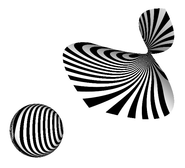
Zebra Stripes applied. |
|---|
|
Environment Map: Also called Reflection Mapping, this method simulates reflection of an environment on a surface, which often helps highlight the object's surface curvature. A default environment map will be used or you can choose another map. |
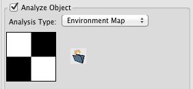
Environment Map options. |
|---|---|
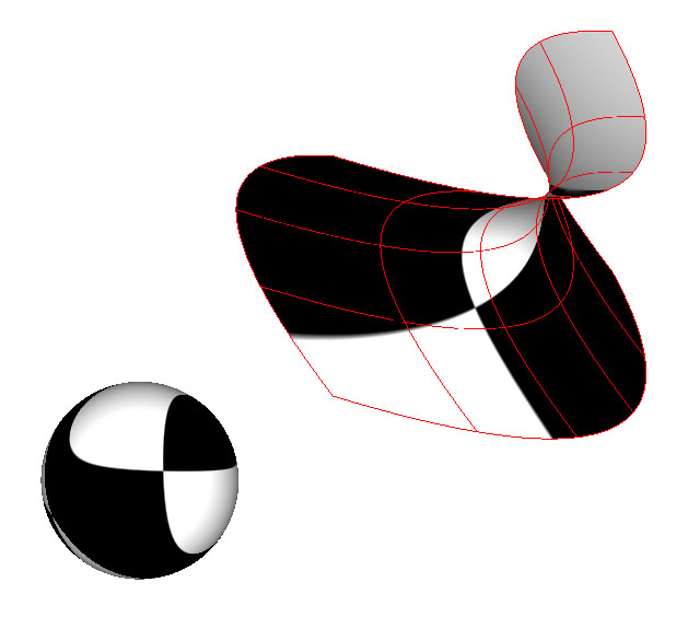
Environment Map applied. |
|
Draft Angle: This color mapping method is used to visualize the angle between the normal to a point of a surface and the active reference plane.
The Minimum Angle field specifies an angle below which the display will be blue. The sliding bar can be used to change the value of this angle or a new value can be typed directly. The Maximum Angle field specifies an angle above which the display will be red. Draft angle values between minimum and maximum will be colored in a spectrum running from blue to red.
|
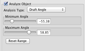
Draft Angle options. |
|---|---|
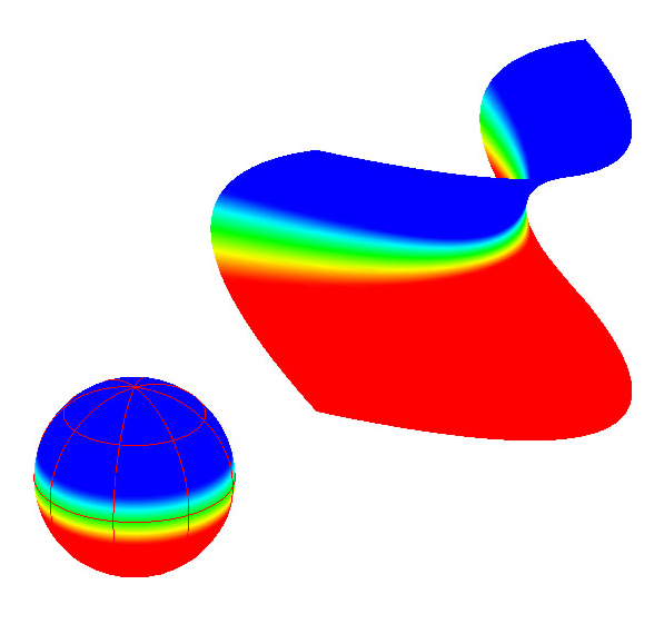
Draft Angle applied. |
|
Curvature Map: This color mapping method provides a visual display of the principal curvatures of a surface.
The Curvature Type popup menu contains six items that specify how curvature should be displayed: Principal Min and Principal Max map the principal minimum and maximum curvature, respectively. Radius Min and Radius Max map the radius of curvature in the principal maximum and minimum direction, respectively. Gaussian maps the product of the principal maximum and minimum curvature. Mean maps the average of the principal maximum and minimum curvature.
The Minimum Radius field specifies a curvature or radius value below which the display will be blue. The Maximum Radius field specifies a curvature or radius value above which the display will be red. Curvature values between minimum and maximum will be colored in a spectrum running from blue to red.
Clicking on the Optimal Range button calculates a range suitable for the selected objects. |
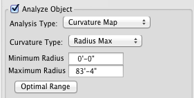
Curvature Environment Map options.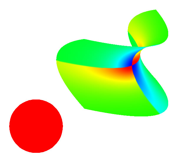
Curvature Map applied. |
|---|
|
Normal Map: Surface normal color mapping provides a visual display of normal direction. Each axis X,Y,Z has an associated color red, green, blue. Surface points will be colored according to the contribution of each axis to the direction of the associated normal.
When the Use Analysis Display Resolution box is checked, the object's standard faceting will be overridden by faceting specifically designed for surface analysis display. This is accomplished through a special Faceting Scheme that is called Surface Analysis. If the object being analyzed does not appear to have enough facets to generate meaningful results, you can increase the density by editing the scheme in the Faceting Schemes section of the Project Settings dialog. Likewise if the object becomes too slow to manipulate because of its increased faceting, you can reduce the faceting in the same manner. When Use Analysis Display Resolution is dialed, the object's current faceting is used for the analysis display. |
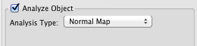
Normal Map has no options.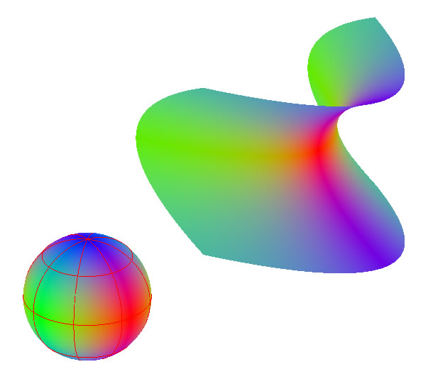
Normal Map applied. |
|---|
|
Porcupine Plot: This is a visual curvature analysis technique for curves and surfaces which places visual “quills” at points along a curve, an edge, or an iso-curve of a surface. The direction of the quill at a point on a curve is determined by the Frenet frame of the curve, while the relative length of the quill reflects the curvature value at that point. The greater the curvature of the curve at the quill point (i.e. the smaller the radius of curvature) the longer the length of the quill. An outer boundary curve is displayed along the tips of the quills.
A Frenet Frame is a set of axes set at each point of a curve that define a coordinate system. As a frame moves along a curve, it rotates in space according to the direction and curvature of the curve.
Parallel quills at a curve boundary indicate G1 continuity, while parallel quills of equal length (assuming equal display magnitudes on all curves) indicates G2 continuity. Parallel quills with equal length and a smooth outer boundary curve indicates G3 continuity. Unlike the faux color surface analysis methods, which are based on primary curvature values, Porcupine Plot uses curvature data along the U and V directions of surfaces.
Porcupine Plot analysis is affected by the following parameters. When these are changed, the porcupine plot is dynamically updated on the screen, whenever Shaded Work or Wire frame rendering mode is used.
Quill Color and Curve Color specify the display colors of the “quills” and the boundary curve, respectively.
When Edges is checked, porcupine plots will be displayed for all edges of smooth objects. U and V Isolines specify the number of interior U and V iso-curves of each face for which a porcupine plot is displayed.
Quill Resolution specifies the number of quills that will be displayed between each knot of a curve. This value can be changed either through the sliding bar or by typing a value in the field.
Quill Scale specifies the relative display scale for the quills.
When Reverse Quill Direction is on, the quill direction is reversed. |
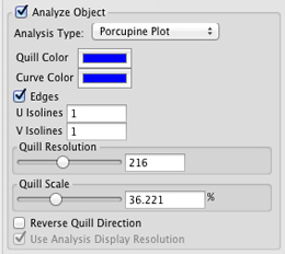
Porcupine Plot options.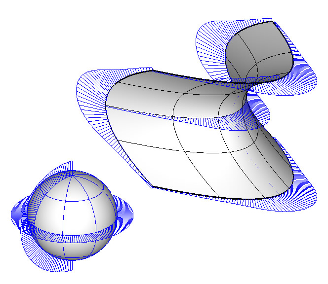
Porcupine Plot applied. |
|---|
