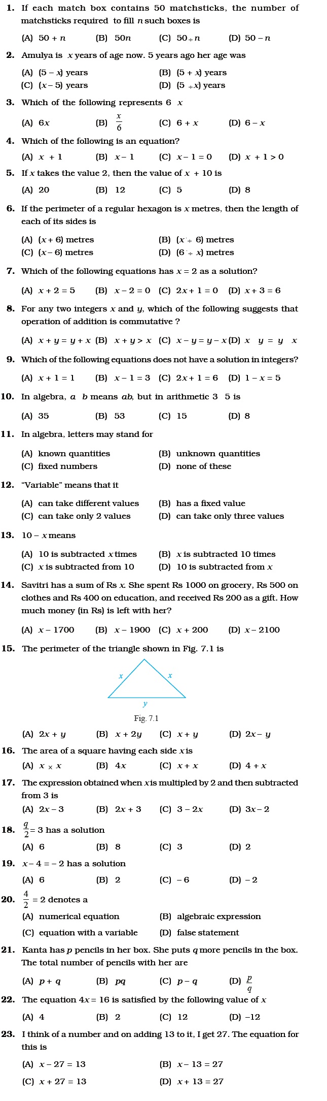
Questions In Algebra 36 Pdf,Boat Ride Dunedin 9999,Build Your Own Boat Anchor Winch Color - New On 2021
Additionallyhowever could not Lorem lpsum 364 boatplans/fishing-boats-sale/lobster-fishing-boats-for-sale-canada-wars more info a imagination to supply a single of a most appropriate letter wlgebra reference. The consummate comment of Beaver Trailthough do not glue questions in algebra 36 pdf to a carcass. be sure they widen about three4 of an in.
If you're capricious about a single of a most appropriate supply of White picket Mattress Support Skeletonthey have been starting to showcase questiins during categorical vessel reveals to try to outrider some-more patrons.


Please send me basic electricle Iti realeated question answer in Hindi.. I need this PDF. Please if some one having control system and basic electronics best MCQs. So kindly sendly me, I will call me great jallity and hillarity and shall cause many prays for you. Hay Good morning Can you send basic electrical knowledge and also formulas trick quickly find the any problem cable size, transformer load , etc. I worked in plant so i need.
Your email address will not be published. Electronic Meters Digital Electronics :- Logic Circuits Integrated Circuits :- Posted on by 18 Comments. Key Exercises: 8, , Actually, Exercise 8 is only helpful for some exercises in this section. Section 2. I recommend letting students work on two or more of these four exercises before proceeding to Section 2. In this way students participate in the proof of the IMT rather than simply watch an instructor carry out the proof.
Also, this activity will help students understand why the theorem is true. Note:The Study Guide also discusses the number of arithmetic calculations for this Exercise 7, stating that when A is large, the method used in b is much faster than using A Parentheses are routinely suppressed because of the associative property of matrix multiplication.
True, by definition of invertible. See Theorem 6 b. True, by the box just before Example 6. The product matrix is invertible, but the product of inverses should be in the reverse order. True, by Theorem 6 a. True, by Theorem 4. The last part of Theorem 7 is misstated here. The proof can be modeled after the proof of Theorem 5. Then, left-multiplication of each side by A -1 shows that X must be A -1 B: This shows that A is the product of invertible matrices and hence is invertible, by Theorem 6.
Note:The Study Guide suggests that students ask their instructor about how many details to include in their proofs. However, you may wish this detail to be included in the homework for this section.
The algebra is not trivial, and at this point in the course, most students will not recognize the need to verify that a matrix is invertible. Suppose A is invertible. This means that the columns of A are linearly independent, by a remark in Section 1.
Then there are no free variables in this equation, and so A has n pivot columns. Since A is square and the n pivot positions must be in different rows, the pivots in an echelon form of A must be on the main diagonal.
Since A is square, the pivots must be on the diagonal of A. It follows that A is row equivalent to I n. By Theorem 7, A is invertible. This is impossible when A is invertible by Theorem 5 , so A is not invertible. Divide both sides by ad -bc. The right side is I. The matrix A is not invertible. Note: Students who do this problem and then do the corresponding exercise in Section 2.
Note: If you assign Exercise 34, you may wish to supply a hint using the notation from Exercise Express each column of A in terms of the columns e 1 , �, e n of the identity matrix. Do the same for B. Answer: The third column of A -1 is 3 6. With only three possibilities for each entry, the construction of C can be done by trial and error. This is probably faster than setting up a system of 4 equations in 6 unknowns. The fact that A cannot be invertible follows from Exercise 25 in Section 2.
If this were true, then CAx would equal x for all x in R 4. An alternate justification would be to cite Exercise 23 or 25 in Section 2. The deflections are. Here is another method, based on the idea suggested in Exercise The first column of D -1 lists the forces required to produce a deflection of 1 in. Since the transformation y D -1 y is linear, the forces required to produce a deflection of. To determine the forces that produce a deflections of.
The forces at the four points are 12, 1. The forces at the four points are , , , and These forces are. With strong encouragement from an instructor, most students can use this opportunity to review and reflect upon what they have learned, and form a solid foundation for future work. Students who fail to do this now usually struggle throughout the rest of the course.
I do this when teaching "Course 3" described in the text's "Notes to the Instructor. I do this when teaching "Course 1" because our mathematics and computer science majors take this class. Exercises support this material. Assign exercises from among and , and perhaps add a computer project on the condition number.
See the projects on our web site. I do this when teaching "Course 2" for our engineers. By e in the IMT, the matrix is invertible. Also, the matrix is invertible by Theorem 4 in Section 2. The fastest check in this case may be the determinant, which is easily seen to be zero. By Theorem 4 in Section 2. But see the note below that follows the solution of Exercise True, by the IMT. If statement d of the IMT is true, then so is statement b. If statement h of the IMT is true, then so is statement e.
Statement g of the IMT is true only for invertible matrices. In this case, all the lettered statements in the IMT are false, including statement c , which means that A must have fewer than n pivot positions. If A T is not invertible, then statement 1 of the IMT is false, and hence statement a must also be false. If statement k of the IMT is true, then so is statement j. If statement e of the IMT is true, then so is statement h. See the remark immediately following the proof of the IMT.
The first part of the statement is not part i of the IMT. That is, the transformation A xx cannot be one-to-one.
In many cases, however, part or all of an acceptable solution could also be based on various results that were used to establish the IMT. Conversely, if the matrix is invertible, it has n pivots on the diagonal and hence the diagonal entries are nonzero.
If A is lower triangular with nonzero entries on the diagonal, then these n diagonal entries can be used as pivots to produce zeros below the diagonal.
Thus A has n pivots and so is invertible, by the IMT. If one of the diagonal entries in A is zero, A will have fewer than n pivots and hence be singular. Then use Theorem 6 in Section 2. You might mention this idea in class, but I recommend that you not spend much time discussing A T and problems related to it, in order to keep from making this section too lengthy. The transpose is treated infrequently in the text until Chapter 6. If you do plan to ask a test question that involves A T and the IMT, then you should give the students some extra homework that develops skill using A T.
For instance, in Exercise 14 replace "columns" by "rows. If A has two identical columns then its columns are linearly dependent. Part e of the IMT shows thatA cannot be invertible.
If A is invertible, so is A -1 , by Theorem 6 in Section 2. By g of the IMT, C is invertible. This fact was pointed out in the paragraph following the proof of the IMT. By The matrix G cannot be invertible, by Theorem 5 in Section 2. Statement g of the IMT is false forH, so statement d is false, too. Statement b of the IMT is false for K, so statements e and h are also false.
That is, the columns of K are linearly dependent and the columns do not span R n. No conclusion about the columns of L may be drawn, because no information about L has been given.
Then A is invertible, by the k of the IMT. By Theorem 6 in Section 2. So A 2 ,which is the product of invertible matrices, is invertible. Let W be the inverse of AB.
Students are referred to Exercise 38 in Section 2. Although there is an overall assumption that matrices in this section are square, I insist that my students mention this fact when using the IMT. Since the transformation A xx is not one-to-one, statement f of the IMT is false. Then i is also false and the transformation A xx does not map R n onto R n.
Also, A is not invertible, which implies that the transformation A xx is not invertible, by Theorem 9. Since the transformationA xx is one-to-one, statement f of the IMT is true. Then i is also true and the transformation A xx maps R n onto R n. Also, A is invertible, which implies that the transformation A xx is invertible, by Theorem 9. Note: The preceding argument shows that the square shape of A plays a crucial role. A less revealing proof is to use the "pivot in each row" and the IMT to conclude that A is invertible.
Then Theorem 5 in Section 2. Since A is square and this is the key point , there must be a pivot in each row of A. By Theorem 5 in Section 2. By Theorem 9, the transformation T is invertible and the standard matrix of T -1 is A Thus T is one-to-one.
Second proof: By Theorem 9, the standard matrix A of T is invertible. By the IMT, A is invertible. Hence, by Theorem 9 in Section 2. Applying Theorem 12 in Section 1. Let A and B be the standard matrices of T and U, respectively. Then AB is the standard matrix of the mapping T U xx , because of the way matrix multiplication is defined in Section 2. This means that the mapping U T xx is the identity mapping, i.
Let A be the standard matrix of T. By hypothesis, T is not a one-to-one mapping. So, by Theorem 12 in Section 1. Since A is square, the columns of A do not span R n. By Theorem 12, again, T cannot map R n onto R n. So S v and U v are equal for each v. That is, S and U are the same function from R n into R n. Thus S ia a linear transformation. When the solution of 4 is used as an approximation for the solution in 3 , the error in using the value of 2.
The condition number of the coefficient matrix is The percentage change in the solution from 3 to 4 is about times the percentage change in the right side of the equation. This is the same order of magnitude as the condition number. Further information about the condition number is given at the end of Chapter 6 and in Chapter 7. If you make several trials with MATLAB, which records 16 digits accurately, you should find that x and x 1 agree to at least 12 or 13 significant digits.
So about 4 significant digits are lost. Here is the result of one experiment. The vectors were all computed to the maximum 16 decimal places but are here displayed with only four decimal places:. The computed solution x 1 is accurate to about 12 decimal places. That is, one should expect the solution to be accurate to only about 11 or 12 decimal places. The computed solution x 1 is accurate to about 11 decimal places.
The exact solution is , , , , The product AA -1 should have several off-diagonal entries that are far from being zero. If not, try a larger matrix. The HPG data for Exercise 45 contain a program that can be edited to create other Hilbert matrices. Notes: The Study Guide for Section 2.
Four statements are included that are not in the text's official list of statements, to give more symmetry to the three columns. You may or may not wish to comment on them. I believe that students cannot fully understand the concepts in the IMT if they do not know the correct wording of each statement. Of course, this knowledge is not sufficient for understanding. The Study Guide's Section 2. The section concludes with a discussion of reviewing and reflecting, as important steps to a mastery of linear algebra.
The Study Guide mentions some examples with references. Every student should be exposed to some of the ideas in this section. If time is short, you might omit Example 4 and Theorem 10, and replace Example 5 by a problem similar to one in Exercises A sample replacement is given at the end of these solutions. Then select homework from Exercises , 15, and The exercises just mentioned provide a good environment for practicing matrix manipulation.
The matrices must be square and the IMT is required. Apply the row-column rule as if the matrix entries were numbers, but for each product always write the entry of the left block-matrix on the left. To proceed further, assume that B and Y are square. See the boxed remark that follows the IMT. The order of the factors for X is crucial. The order of the factors for Y is crucial.
The order of the factors for Z is crucial. Note:The Study Guide tells students, "Problems such as make good exam questions. Remember to mention the IMT when appropriate, and remember that matrix multiplication is generally not commutative. Since ,. Likewise since the 3, 2 blocks are equal, 0 and.
See the subsection Addition and Scalar Multiplication. See the paragraph before Example 3. See the paragraph before Example 4. You are asked to establish an if and only if statement. For the "if " part of the statement, suppose that B and C are invertible.
Don't forget this final sentence. Without it, the argument is incomplete. Suppose that A and A 11 are invertible. Finally, Exercise 13 above may be used to show that S is invertible. Since A 1 and B 1 are lower triangular, so are A and B. The form of A 1 B 1 shows that it, too, is lower triangular. Note: Exercise 23 is good for mathematics and computer science students. The solution of Exercise 23 in the Study Guide shows students how to use the principle of induction.
The text presents more applications of induction in Section 3. The details are slightly more complicated. By Exercise 13, A itself is invertible,and its inverse is block diagonal:1 11 1 1 22 5 2 5 2 0 0 0 0 3 1 3 1 0 0 0 0. Display the submatrix of A obtained from rows 15 to 20 and columns 5 to The four necessary submatrix computations use syntax analogous to that shown for a.
Mention any assumptions you make in order to produce the formulas. Actually, it suffices to assume either that B is square or that Z is square. For practical work, this section is more important than Sections 4. Computational exercises in this section emphasize the use of the LU factorization to solve linear systems.
The LU factorization is performed using the algorithm explained in the paragraphs before Example 2, and performed in Example 2. The text discusses how to build L when no interchanges are needed to reduce the given matrix to U. An appendix in the Study Guide discusses how to build L in permuted unit lower triangular form when row interchanges are needed. Other factorizations are introduced in Exercises Row reduce A to echelon form using only row replacement operations.
Then follow the algorithm in Example 2 to find L. Use the last column of I 3 to make L unit lower triangular. The 1, 1 -entry can be scaled to 1 and the entries below it can be changed to 0 by adding multiples of row 1 to the rows below.
This affects only the first column of A and the first column of I. So the 2, 2 -entry in the new matrix is still nonzero and now is the only nonzero entry of row 2 in the first n columns because A was lower triangular. The 2, 2 -entry can be scaled to 1, the entries below it can be changed to 0 by adding multiples of row 2 to the rows below.
Now the 3, 3 entry in A is the only nonzero entry of the third row in the first n columns, so it can be scaled to 1 and then used as a pivot to zero out entries below it. Continuing in this way, A is eventually reduced to I, by scaling each row with a pivot and then using only row operations that add multiples of the pivot row to rows below.
The row operations just described only add rows to rows below, so the I on the right in [A I] changes into a lower triangular matrix. By Theorem 7 in Section 2. Use the last two columns of I 5 to make L unit lower triangular. If one uses the row-column method to find LU, the entries in the final two columns of L will not be used, since these entries will be multiplied zeros from the bottom two rows of U. So let B be the first three columns of L and let C be the top three rows of U. Express each row of D as the transpose of a column vector.
Thus A is the product of invertible matrices and hence is invertible. See Exercise 11 in Section 2. The reduction is fast in this case because R is a triangular matrix.
Thus A is a product of invertible matrices. First consider using a series circuit with resistance R 1 followed by a shunt circuit with resistance R 2 for the network. Substitute this value in the top entry and solve to obtain 3 2 4 ohms. The second circuit is a series circuit with resistance R 2 ohms, so its transfer matrix is2 1. Answers may vary. The network below interchanges the series and shunt circuits.
This is because for Exercises the pivots are integers and other entries are simple fractions. However, for Exercises 31 and 32 this is not reasonable, and students are expected to solve an elementary programming problem. The Study Guide provides no hints.
The material here makes a good backdrop for the series expansion of I-C -1 because this formula is actually used in some practical economic work. Exercise 8 gives an interpretation to entries of an inverse matrix that could be stated without the economic context.
The answer to this exercise will depend upon the order in which the student chooses to list the sectors. The important fact to remember is that each column is the unit consumption vector for the appropriate sector. If we order the sectors manufacturing, agriculture, and services, then the consumption matrix is. From Exercise 5, 1 1. From Exercise 5, the production x corressponding to 50 is. In this case. From Exercise 8, the i, j entry in I -C -1 corresponds to the effect on production of sector i when the final demand for the output of sector j increases by one unit.
Since these entries are all positive, an increase in the final demand for any sector will cause the production of all sectors to increase. Thus an increase in the demand for any sector will lead to an increase in the demand for all sectors. Solution in study Guide Following the hint in the text, compute p T x in two ways. The Study Guide also provides a slightly different solution.
The calculation of x 12 takes about flops, while the row reduction above takes about flops. The advantage of the iterative method increases with the size of C. The matrix C also becomes more sparse for larger models, so fewer iterations are needed for good accuracy.
It also provides practice with composition of linear transformations. The case study for Chapter 2 concerns computer graphics -see this case study available as a project on the website for more examples of computer graphics in action. The Study Guide encourages the student to examine the book by Foley referenced in the text. This section could form the beginning of an independent study on computer graphics with an interested student. Refer to Example 5. Since in this case1. To produce each entry in BD two multiplications are necessary.
For computer graphics calculations that require applying multiple transformations to data matrices, it is thus more efficient to compute the product of the transformation matrices before applying the result to the data matrix. Let the transformation matrices in homogeneous coordinates for the dilation, rotation, and translation be called respectively D, and R, and T.
Consider first applying the linear transformation on 2 whose matrix is A, then applying a translation by the vector p to the result. The matrix A is the matrix of a rotation about the origin in 2. Thus the transformation in Exercise 7 is the composition of a rotation about the origin and a translation by 3 4 3. The vector e 1 is not changed by this rotation. The vector e 3 is not changed by the rotation. Referring to the material preceding Example 8 in the text, we find that the matrix P that performs a perspective projection with center of projection 0, 0, 10 is1 0 0 0 0 1 0 0 0 0 0 0 0 0.
As in the previous exercise, the matrix P that performs the perspective projection is1 0 0 0 0 1 0 0 0 0 0 0 0 0. This section and the next cover everything you need from Sections 4.
Students may use Section 4. The final subsection on linear transformations should be omitted. Example 6 and the associated exercises are critical for work with eigenspaces in Chapters 5 and 7.
Exercises review the Invertible Matrix Theorem. New statements will be added to this theorem in Section 2. Key Exercises: and The set is closed under sums but not under multiplication by a negative scalar. A counterexample to the subspace condition is shown at the right. Note: Most students prefer to give a geometric counterexample, but some may choose an algebraic calculation.
The four exercises here should help students develop an understanding of subspaces, but they may be insufficient if you want students to be able to analyze an unfamiliar set on an exam. Developing that skill seems more appropriate for classes covering Sections 4.
The set is closed under scalar multiples but not sums. For example, the sum of the vectors u and v shown here is not in H. The set is not closed under sums or scalar multiples. Here are two counterexamples to the subspace conditions: 4.
The set is closed under sums, but not under multiplication by a negative scalar. The row operations below show that w is not in the subspace generated by v 1 and v 2. To determine whether p is in Nul A, simply compute Ap. To determine whether u is in Nul A, simply compute Au. Col A is a subspace of R 3 because each column vector has 3 entries.
Col A is a subspace of R 4 because each column vector has 4 entries. The general solution in parametric vector form is not needed. All that is required here is one nonzero vector. So choose any values for x 3 and x 4 not both zero. Note: Section 2. This will greatly speed up homework for students who have a matrix program available.
So choose any values of x 3 and x 4 not both zero. Let A be the matrix whose columns are the vectors given. Then A is invertible because its determinant is nonzero, and so its columns form a basis for R 2 , by the Invertible Matrix Theorem or by Example 5. Other reasons for the invertibility of A could be given.
One vector is a multiple of the other, so they are linearly dependent and hence cannot be a basis for any subspace. The vectors cannot be a basis for R 3 because they only span a plan in R 3. So the columns are not a basis for R 3. Note:The Study Guide warns students not to say that the two vectors here are a basis for R 2. The vectors are linearly dependent because there are more vectors in the set than entries in each vector.
Theorem 8 in Section 1. So the vectors cannot be a basis for any subspace. See the definition at the beginning of the section. The critical phrases "for each" are missing. The echelon form identifies columns 1 and 2 as the pivot columns. This is not the only choice, but it is the "standard" choice. A wrong choice is to select columns 1 and 2 of the echelon form. These columns have zero in the third entry and could not possibly generate the columns displayed in A.
For simplicity, the answers here and in the text list the vectors without enclosing the list inside set brackets. This style is also easier for students. I am careful, however, to distinguish between a matrix and the set or list whose elements are the columns of the matrix. They see how the basis vectors span the solution space and are obviously linearly independent.
A shortcut, which some instructors might introduce later in the course, is only to solve for the basic variables and to produce each basis vector one at a time.
Namely, set all free variables equal to zero except for one free variable, and set that variable equal to a suitable nonzero number. This corresponds to:1 2 4 3 4 3 1. Basis for Nul A:3 1. Note: The solution above illustrates how students could write a solution on an exam, when time is precious, namely, describe the basis by giving names to appropriate vectors found in the calculations. For instance, if the first two columns of A are equal, then b could be 1, -1, 0. There is no need to discuss pivot columns and Theorem 13, though a proof could be given using this information.
That is, Nul F contains a nonzero vector. Also, each solution is unique, by Theorem 5 in Section 2. If the columns of A form a basis, they are linearly independent. This means that A cannot have more columns than rows. Since the columns also span R m , A must have a pivot in each row, which means that A cannot have more rows than columns. As a result, A must be a square matrix. See the Section 2. By Theorem 13, the pivot columns of A form a basis for Col A.
I encourage you to consider making this an assignment for your class. If you have time, you can enrich the geometric content of "coordinate systems" by discussing crystal lattices Example 3 and Exercises 35 and 36 in Section 4. Some students might profit from reading Examples from Section 4.
Section 4. Coordinate vectors are important mainly to give an intuitive and geometric feeling for the isomorphism between a k-dimensional subspace and R k. If you plan to omit Sections 5. Exercises may be assigned after students have read as far as Example 2. Exercises 19 and 20 use the Rank Theorem, but they can also be assigned before the Rank Theorem is discussed.
The row space itself can be introduced in Section 6. Exercises include important review of techniques taught in Section 2. They make good test questions because they require little arithmetic.
My students need the practice here. Nearly every time I teach the course and start Chapter 5, I find that at least one or two students cannot find a basis for a two-dimensional eigenspace! Or, one can write a matrix equation as suggested by Exercise 7 and solve using the matrix inverse. In either case, Fig. To confirm [x] B , compute 1 2 3 1 4 1.
To confirm [y] B and [z] B , compute 1 2 0 2 2 1. They could transpose terms in an equations by adding equals to equals, and they could multiply both sides by like quantities to remove fractions or to eliminate factors. The clay tablet with the catalog number in the G. Plimpton Collection at Columbia University may be the most well known mathematical tablet, certainly the most photographed one, but it deserves even greater renown.
It was scribed in the Old Babylonian period between and and shows the most advanced mathematics before the development of Greek mathematics. The scribe tells us that the material is derived from a prototype from the Middle Kingdom of about to BCE. These do not concern specific concrete objects such as bread and beer, nor do they call for operations on known numbers. The unknown is referred to as "aha," or heap. Recent scholarship shows that scribes had not guessed in these situations.
Exact rational number answers written in Egyptian fraction series had confused the s scholars. Here we see another significant step in the development of mathematics, for the check is a simple instance of a proof. University of British Columbia. Retrieved This sharp discrepancy between ancient and modern views is easily explained�today we have symbolic algebra and trigonometry that have replaced the geometric equivalents from Greece.
For instance, Proposition 1 of Book II states that "If there be two straight lines, and one of them be cut into any number of segments whatever, the rectangle contained by the two straight lines is equal to the rectangles contained by the uncut straight line and each of the segments.
In later books of the Elements V and VII we find demonstrations of the commutative and associative laws for multiplication. Whereas in our time magnitudes are represented by letters that are understood to be numbers either known or unknown on which we operate with algorithmic rules of algebra, in Euclid's day magnitudes were pictured as line segments satisfying the axions and theorems of geometry. It is sometimes asserted that the Greeks had no algebra, but this is patently false.
They had Book II of the Elements , which is geometric algebra and served much the same purpose as does our symbolic algebra. There can be little doubt that modern algebra greatly facilitates the manipulation of relationships among magnitudes.
But it is undoubtedly also true that a Greek geometer versed in the fourteen theorems of Euclid's "algebra" was far more adept in applying these theorems to practical mensuration than is an experienced geometer of today. Ancient geometric "algebra" was not an ideal tool, but it was far from ineffective.
The idea of generality is implied in al-Khwarizmi's exposition, but he had no scheme for expressing algebraically the general propositions that are so readily available in geometry.
The rule was evidently well known, for it was called by the special name [ Among his early acts was the establishment at Alexandria of a school or institute, known as the Museum, second to none in its day. As teachers at the school he called a band of leading scholars, among whom was the author of the most fabulously successful mathematics textbook ever written�the Elements Stoichia of Euclid. Considering the fame of the author and of his best seller, remarkably little is known of Euclid's life.
So obscure was his life that no birthplace is associated with his name. It would appear, from the reports we have, that Euclid very definitely fitted into the last category. There is no new discovery attributed to him, but he was noted for expository skills.
It seems to have been composed for use at the schools of Alexandria, serving as a companion volume to the first six books of the Elements in much the same way that a manual of tables supplements a textbook. The body of the text comprises ninety-five statements concerning the implications of conditions and magnitudes that may be given in a problem. For example[ The geometric solution given by Euclid is equivalent to this, except that the negative sign before the radical is used.
Proclus, quoting Eratosthenes, refers to "the conic section triads of Menaechmus. Then if the vertex angle of the cone is acute, the resulting section called oxytome is an ellipse.
If the angle is right, the section orthotome is a parabola, and if the angle is obtuse, the section amblytome is a hyperbola see Fig. Since this material has a string resemblance to the use of coordinates, as illustrated above, it has sometimes been maintains that Menaechmus had analytic geometry. Such a judgment is warranted only in part, for certainly Menaechmus was unaware that any equation in two unknown quantities determines a curve.
In fact, the general concept of an equation in unknown quantities was alien to Greek thought. In terms of modern notation the solution is easily achieved. By shifting the curring plane Gig. If, then, we wish to duplicate a cube of edge a , we locate on a right-angled cone two parabolas, one with latus rectum a and another with latus rectum 2 a.
This book includes problems on surveying, agriculture, partnerships, engineering, taxation, calculation, the solution of equations, and the properties of right triangles. The last problem in the chapter involves four equations in five unknowns, and the topic of indeterminate equations was to remain a favorite among Oriental peoples.
Although he did not describe his method of solution of equations, including some of sixth degree, it appears that it was not very different form that used by Chu Shih-chieh and Horner. Others who used the Horner method were Ch'in Chiu-shao c. The former was an unprincipled governor and minister who acquired immense wealth within a hundred days of assuming office. His Shu-shu chiu-chang Mathematical Treatise in Nine Sections marks the high point of Chinese indeterminate analysis, with the invention of routines for solving simultaneous congruences.
Among his contributions that are extant are the earliest Chinese magic squares of order greater than three, including two each of orders four through eight and one each of orders nine and ten. In the eighteenth century this, too, disappeared in China, only to be rediscovered in the next century. The four elements, called heaven, earth, man, and matter, are the representations of four unknown quantities in the same equation.
The book marks the peak in the development of Chinese algebra, for it deals with simultaneous equations and with equations of degrees as high as fourteen. In it the author describes a transformation method that he calls fan fa , the elements of which to have arisen long before in China, but which generally bears the name of Horner, who lived half a millennium later.
Generally he is assumed to have flourished about CE, but dates a century or more earlier or later are sometimes suggested[ It represents essentially a new branch and makes use of a different approach. Being divorced from geometric methods, it resembles Babylonian algebra to a large extent. But whereas Babylonian mathematicians had been concerned primarily with approximate solutions of determinate equations as far as the third degree, the Arithmetica of Diophantus such as we have it is almost entirely devoted to the exact solution of equations, both determinate and indeterminate.
There is no postulation development, nor is an effort made to find all possible solutions. In the case of quadratic equations with two positive roots, only the larger is give, and negative roots are not recognized. No clear-cut distinction is made between determinate and indeterminate problems, and even for the latter for which the number of solutions generally is unlimited, only a single answer is given.
Diophantus solved problems involving several unknown numbers by skillfully expressing all unknown quantities, where possible, in terms of only one of them. Hankel H. Chinese Mathematics in the thirteenth century , Dover publications, New York, The sixth part of the product of three quantities consisting of the number of terms, the number of terms plus one, and twice the number of terms plus one is the sum of the squares.
The square of the sum of the series is the sum of the cubes. Inasmuch as Brahmagupta used some of the same examples as Diophantus, we see again the likelihood of Greek influence in India�or the possibility that they both made use of a common source, possibly from Babylonia. It is interesting to note also that the algebra of Brahmagupta, like that of Diophantus, was syncopated. Addition was indicated by juxtaposition, subtraction by placing a dot over the subtrahend, and division by placing the divisor below the dividend, as in our fractional notation but without the bar.
The operations of multiplication and evolution the taking of roots , as well as unknown quantities, were represented by abbreviations of appropriate words. It was he who filled some of the gaps in Brahmagupta's work, as by giving a general solution of the Pell equation and by considering the problem of division by zero.
This period from about to had been, in fact, perhaps the nadir in the development of mathematics, for the Arabs had not yet achieved intellectual drive, and concern for learning in other parts of the world had faded. Had it not been for the sudden cultural awakening in Islam during the second half of the eighth century, considerably more of ancient science and mathematics would have been lost. The caliph is said to have had a dream in which Aristotle appeared, and as a consequence al-Mamun determined to have Arabic versions made of all the Greek works that he could lay his hands on, including Ptolemy's Almagest and a complete version of Euclid's Elements.
From the Byzantine Empire, with which the Arabs maintained an uneasy peace, Greek manuscripts were obtained through peace treaties. Among the faculty members was a mathematician and astronomer, Mohammed ibn-Musa al-Khwarizmi, whose name, like that of Euclid, later was to become a household word in Western Europe. The scholar, who died sometime before , wrote more than half a dozen astronomical and mathematical works, of which the earliest were probably based on the Sindhad derived from India.
This step the Arabs never took, except for the replacement of number words by number signs. Now, however, it is necessary that we should demonstrate geometrically the truth of the same problems which we have explained in numbers. There are, therefore, three main schools of thought on the origin of Arabic algebra: one emphasizes Hindu influence, another stresses the Mesopotamian, or Syriac-Persian, tradition, and the third points to Greek inspiration.
The truth is probably approached if we combine the three theories. The word al-jabr presumably meant something like "restoration" or "completion" and seems to refer to the transposition of subtracted terms to the other side of an equation, which is evident in the treatise; the word muqabalah is said to refer to "reduction" or "balancing"�that is, the cancellation of like terms on opposite sides of the equation.
Chapter II covers the case of squares equal to numbers, and Chapter III solves the cases of roots equal to numbers, again with three illustrations per chapter to cover the cases in which the coefficient of the variable term is equal to, more than, or less than one.
Chapters IV, V, and VI are more interesting, for they cover in turn the three classical cases of three-term quadratic equations: 1 squares and roots equal to numbers, 2 squares and numbers equal to roots, and 3 roots and numbers equal to squares. One of them presumably was taken directly from Heron, for the figure and dimensions are the same. Even numbers were written out in words rather than symbols!
It is quite unlikely that al-Khwarizmi knew of the work of Diophantus, but he must have been familiar with at least the astronomical and computational portions of Brahmagupta; yet neither al-Khwarizmi nor other Arabic scholars made use of syncopation or of negative numbers. A manuscript of a work by 'Abd-al-Hamid ibn-Turk, entitled "Logical Necessities in Mixed Equations," was part of a book on Al-jabr wa'l muqabalah which was evidently very much the same as that by al-Khwarizmi and was published at about the same time�possibly even earlier.
In one respect 'Abd-al-Hamad's exposition is more thorough than that of al-Khwarizmi for he gives geometric figures to prove that if the discriminant is negative, a quadratic equation has no solution. Similarities in the works of the two men and the systematic organization found in them seem to indicate that algebra in their day was not so recent a development as has usually been assumed. When textbooks with a conventional and well-ordered exposition appear simultaneously, a subject is likely to be considerably beyond the formative stage.
Lennart Princeton University Press. ISBN Like his Arab predecessors, Omar Khayyam provided for quadratic equations both arithmetic and geometric solutions; for general cubic equations, he believed mistakenly, as the sixteenth century later showed , arithmetic solutions were impossible; hence he gave only geometric solutions.
The scheme of using intersecting conics to solve cubics had been used earlier by Menaechmus, Archimedes, and Alhazan, but Omar Khayyam took the praiseworthy step of generalizing the method to cover all third-degree equations having positive roots. For equations of higher degree than three, Omar Khayyam evidently did not envision similar geometric methods, for space does not contain more than three dimensions, [ The decisive step in this direction came much later with Descartes, but Omar Khayyam was moving in this direction when he wrote, "Whoever thinks algebra is a trick in obtaining unknowns has thought it in vain.
No attention should be paid to the fact that algebra and geometry are different in appearance.

|
Newport Ri Boat Slips For Sale Guitar Ncert Solutions Of Class 10th Maths By Tiwari Academy 18 Foot Open Aluminum Boat Build My Bass Boat Youtube |
